Astonishing approximations
Intro
The misconception that all maths problems can be neatly solved with pen and paper stems from the emphasis of traditional education on exactness and formulaic problem-solving. This limited view overlooks the reality that numerous real-world maths scenarios resist closed-form solutions and can only be tackled approximately. Scientists often resort to approximation techniques, numerical algorithms, or computational methods to obtain close estimations rather than exact answers.
In this post I will introduce some basic ideas related to a general mathematical framework for dealing with certain types of problems that evade precise resolution. These ideas belong to an area of applied mathematics usually referred to as perturbation theory. Rather than attempting to provide a comprehensive definition of this field, I will focus exclusively on just one particular example that illustrates some of its characteristic features.
The problem
Typically, problems in pertubation theory depend on a very small (or very large) parameter. In what follows $\varepsilon$ will denote a very small such non-dimensional quantity. The problem we will be concerned with is that of finding approximations for the roots of the cubic
\[y = x^3-2x^2+\varepsilon{x}. \tag{1}\]Although this cubic can be solved by hand, we will ignore that for the moment. The method discussed below can be applied to large classes of cubics for which closed-form solutions are unavailable.
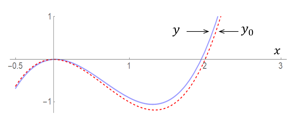
Initially, one might consider the equation with $\varepsilon=0$. In this case $y\simeq y_0$, where
\[y_0 = x^3-2x^2.\]The roots of this equation can be easily found by solving $x^2(x-2)=0$ – hence, $x=2$ and $x=0$ (with a repeated root).

The graphs of the two functions are quite close to each other. Visual inspection confirms that one of the roots of $y(x)=0$ will be close to $x=2$, but near the origin the situation is more complicated since $x=0$ is not a repeated root of (1). We are going to deal with the former case first.
The root away from the origin
Guided by the above observations, we look for an approximation of the root of (1) near $x=2$ with an expression of the form
\[x = 2+a\varepsilon + b\varepsilon^2+\dots, \tag{2}\]where $a$, $b\in\mathbb{R}$ are constants that we aim to find. Also, the dots in (2) denote higher-order terms that will not be needed for our immediate purposes (these are terms involving powers of $\varepsilon^3$, $\varepsilon^4$, and so on).
The next step is to substitute (2) into $x^3-2x^2+\varepsilon{x}=0$, collect together like powers of $\varepsilon$, and then set to zero their corresponding coefficients. This gives
\[\begin{aligned}[t] (2+a\varepsilon + b\varepsilon^2+\dots)^3 &- 2(2+a\varepsilon+b\varepsilon^2+\dots)^2\\ &+\varepsilon(2+a\varepsilon+b\varepsilon^2+\dots) = 0 \end{aligned}\]or
\[(8+12a\varepsilon + \dots)-(8+8a\varepsilon+\dots)+(2\varepsilon+\dots) = 0,\]whence $2\varepsilon(2a+1) = 0$. This gives $a=-1/2$, so the approximation found at this stage is
\[x \simeq 2-\dfrac{1}{2}\varepsilon,\]which is reasonably accurate if $\varepsilon$ is very close to zero (e.g., $\varepsilon=0.01$). With a little bit more work it can be shown that a better approximation is given by
\[x\simeq 2-\dfrac{1}{2}\varepsilon-\dfrac{1}{8}\varepsilon^2-\dfrac{1}{16}\varepsilon^3.\]The root close to the origin
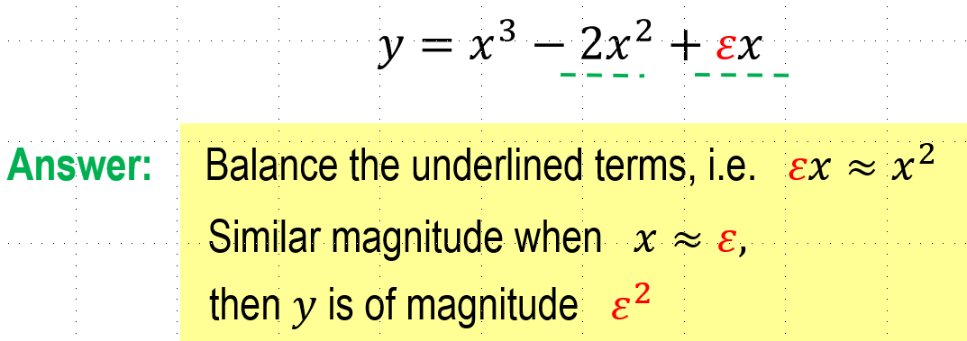
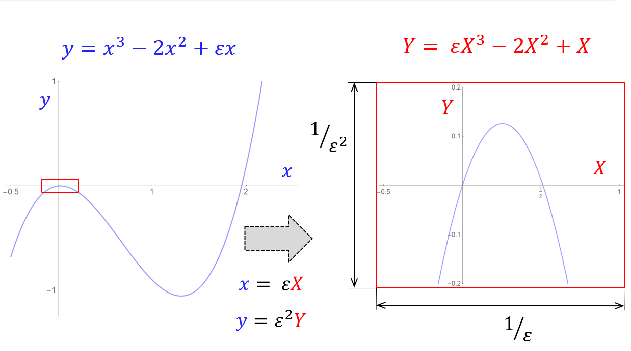
Let’s return now to the other roots near $x=0$. In this situation the approximation $y\simeq y_0$ is unlikely to be very good because we already suspect that the root we are looking for (besides the obvious $x=0$) is likely to be small (this is confirmed by the plot included above). Thus, it is not accurate to neglect the term $\varepsilon{x}$ in our cubic. The key idea is to use the right magnification to better “see” what is going on near the origin; this amounts to re-scaling the original variables (both $x$ and $y$), so that we can zoom in and get better details locally near $x=0$. The obvious question is: how much should we magnify in the x- and y-directions?

The suggested scalings are
\[x = \varepsilon{X}\quad\mbox{and}\quad y=\varepsilon^2{Y}.\]We get something like this

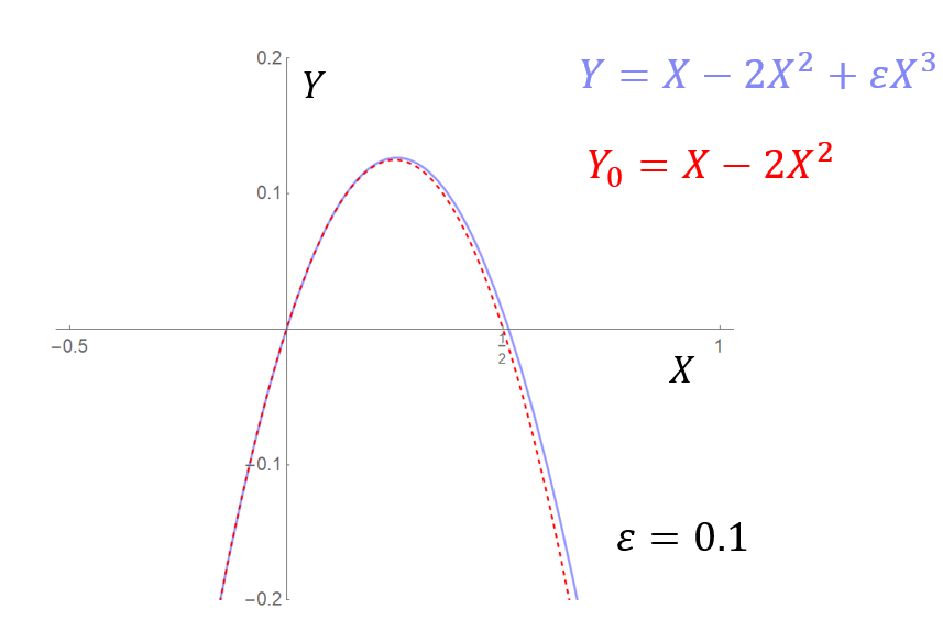
The magnified window (in red) is also shown separately below, where we include both the rescaled cubic and its limiting expression when $\varepsilon=0$. Note that we have essentially reduced the problem to a situation that mirrors closely what we had previously.

The roots of $Y_0$ are at $X=0$ and $X=1/2$ (i.e., at $x=\varepsilon/2$). To find an approximation for the non-zero $X$-root near $X=1/2$, we put
\[X = \dfrac{1}{2}+c\varepsilon + d\varepsilon^2+\dots, \tag{3}\]where $c$, $d\in\mathbb{R}$ are unknown constant at this stage, and the dots have the same connotation as before. The process by which the constants are identified is also identical to what we have done above. The expression (3) is plugged back into $X-2X^2+\varepsilon{X^3}=0$, the like powers of $\varepsilon$ are grouped together, followed by setting to zero their corresponding coefficients. We get
\[(1/2 + c\varepsilon+\dots)-2(1/4+c\varepsilon+\dots) + (\varepsilon/8+\dots) = 0,\]whence $c=1/8$ and our approximation becomes
\[X = \dfrac{1}{2}+\dfrac{1}{8}\varepsilon + \dots.\]In terms of the original cubic, the approximations of the two non-trivial roots are
\[x = \dfrac{1}{2}\varepsilon+\dfrac{1}{8}\varepsilon^2\dots\quad\mbox{and}\quad x = 2-\dfrac{1}{2}\varepsilon+\dots. \tag{4}\]Various comparisons between these predictions and the “exact” values of the roots are included below for $\varepsilon=10^{-1}$ and $\varepsilon=10^{-2}$.

Notes:
A first observation
It is perhaps worth re-iterating that the preceding example was selected to exemplify fundamental concepts in perturbation theory rather than for its inherent complexity. In fact, we can very easily solve this problem by observing that the roots of (1) are $x=0$ and $x=x_{\pm}$, where the latter are given by the quadratic $x^2-2x+\varepsilon=0$, i.e.
\[x_{\pm} = 1\pm(1-\varepsilon)^{1/2}.\]With the help of the general binomial expansion theorem (valid for $| \varepsilon |<1$)
\[(1-\varepsilon)^\alpha = 1-\alpha\varepsilon + \dfrac{\alpha(\alpha-1)}{2!}\varepsilon^2 -\dfrac{\alpha(\alpha-1)(\alpha-2)}{3!}\varepsilon^3 + \dots,\]by taking $\alpha=1/2$ one can easily recover the two formulae in (4). However, the strategy outlined above can be applied to much more complicated situations in which we do not have the luxury of closed-form expressions for the roots of the equation that we want to solve.
A second observation
In searching for the approximation of the roots of the various equations above, we have considered power series in $\varepsilon$, i.e. expressions of the form
\[a_0 + a_1\varepsilon + a_2\varepsilon^2+\dots \equiv\sum_{k=1}^\infty a_k\varepsilon^k, \tag{5}\]where the coefficients $a_k\in\mathbb{R}$ ($k=1,2,\dots$) are determined as part of the solution. This was a direct consequence of the fact that the roots we were looking for were regular (i.e., differentiable) functions of $\varepsilon$ in a small vicinity of $\varepsilon=0$. In many situations this is no longer true, and one has to allow for more generality in (5); e.g., negative and/or fractional exponents.
An example that illustrates the above remark is the cubic
\[x^3-\varepsilon{x} + 2\varepsilon^2 = 0, \tag{6}\]where $\varepsilon>0$ is a (very) small given parameter. Using similar arguments as those outlined in this post, one can show that the three real roots of (6) admit the approximations
\[\begin{aligned}[t] &x_1 = -\varepsilon^{1/2}-\varepsilon+\dfrac{3}{2}\varepsilon^{3/2}-4\varepsilon^2 +\dfrac{105}{8}\varepsilon^{5/2}-\dots,\\ &{}\\ &x_2 = \varepsilon^{1/2}-\varepsilon-\dfrac{3}{2}\varepsilon^{3/2}-4\varepsilon^2 -\dfrac{105}{8}\varepsilon^{5/2}-\dots,\\ &{}\\ &x_3 = 2\varepsilon + 8\varepsilon^2 + 96\varepsilon^3 + \dots, \end{aligned}\]where the dots stand for higher fractional powers of $\varepsilon$.
If we slightly amend (6), i.e. we change the sign in front of the $\varepsilon{x}$ term so that now $x^3+\varepsilon{x} + 2\varepsilon^2 = 0$, then two of the roots are complex conjugate and
\[\begin{aligned}[t] &x_1 = -{\mathrm{i}}\varepsilon^{1/2}+\varepsilon-\dfrac{3}{2}{\mathrm{i}}\varepsilon^{3/2} -4\varepsilon^2 +\dfrac{105}{8}{\mathrm{i}}\varepsilon^{5/2}+\dots,\\ &{}\\ &x_1 = {\mathrm{i}}\varepsilon^{1/2}+\varepsilon+\dfrac{3}{2}{\mathrm{i}}\varepsilon^{3/2} -4\varepsilon^2 -\dfrac{105}{8}{\mathrm{i}}\varepsilon^{5/2}+\dots,\\ &{}\\ &x_3 = -2\varepsilon + 8\varepsilon^2 - 96\varepsilon^3 + \dots, \end{aligned}\]with ${\mathrm{i}}\equiv\sqrt{-1}$ the usual imaginary unit.
Power series with fractional exponents are sometimes called Puisseux series (but the theory of these complicated mathematical objects is not really needed in a serious way in perturbation theory).
A good elementary treatment of pertubation theory can be found in 1, while Murdock 2 provides a more detailed mature discussion regarding the approximations of roots for various polynomials. Nayfeh 3 presents the same topic in a student-friendly format with lots of solved examples and a rich selection of practice questions; the solutions to these, together with additional material, are included in another text by the same author 4.
Footnotes
-
Simmonds, J.G., Mann, J.E.: A First Look at Perturbation Theory (2nd ed.). Dover Publications, Mineola NY (1998). ↩
-
Murdock, J.A.: Perturbations: Theory and Methods. SIAM, Philadelphia (1999). ↩
-
Nayfeh, A.H.: Introduction to Perturbation Theory. John Wiley & Sons, New York (1981). ↩
-
Nayfeh, A.H.: Problems in Perturbation. John Wiley & Sons, New York (1985). ↩